Graphing the Sine and Cosine Functions
Learning Objective(s)
· Determine the coordinates of points on the unit circle.
· Graph the sine function.
· Graph the cosine function.
· Compare the graphs of the sine and cosine functions.
Introduction
You know how to graph many types of functions. Graphs are useful because they can take complicated information and display it in a simple, easy-to-read manner. You’ll now learn how to graph the sine and cosine functions, and see that the graphs of the sine function and cosine function are very similar.
We have seen a point (x,y) on a graph of a function. The first coordinate is the input or value of the variable, and the second coordinate is the output or value of the function.
Each point on the graph of the sine function will have the form ![]() , and each point on the graph of the cosine function will have the form
, and each point on the graph of the cosine function will have the form ![]() . It is customary to use the Greek letter theta,
. It is customary to use the Greek letter theta, ![]() , as the symbol for the angle. Graphing points in the form
, as the symbol for the angle. Graphing points in the form ![]() is just like graphing points in the form (x, y). Along the x-axis we will be plotting
is just like graphing points in the form (x, y). Along the x-axis we will be plotting ![]() , and along the in the y-axis we will be plotting the value of
, and along the in the y-axis we will be plotting the value of ![]() . The graphs that we’ll draw will use values of
. The graphs that we’ll draw will use values of ![]() in radians. Before drawing the graphs, it’ll be useful to find some values of
in radians. Before drawing the graphs, it’ll be useful to find some values of ![]() and
and ![]() , and then gather them together in a table.
, and then gather them together in a table.
Let’s review the general definitions of these functions. Given any angle ![]() , draw it in standard position together with a unit circle. The terminal side will intersect the circle at some point
, draw it in standard position together with a unit circle. The terminal side will intersect the circle at some point ![]() , as shown below.
, as shown below.
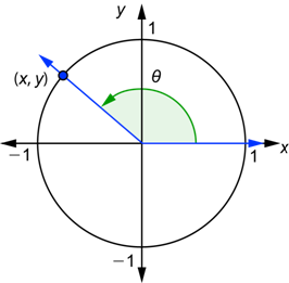
The value of ![]() has been defined to be the x-coordinate of this point, and the value of
has been defined to be the x-coordinate of this point, and the value of ![]() has been defined to be the y-coordinate of this point.
has been defined to be the y-coordinate of this point.
| Example | ||
| Problem | Find the values of | |
|
|
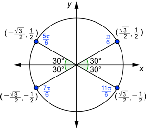
| You might find it useful to convert these angles to degrees. All four angles have a reference angle of 30° or |
|
|
| Use the right triangle definition to find the |
|
|
| Graph the four angles in standard position. The coordinates of the point in the first quadrant were found above. The x-coordinate is the value of cos θ, and the y-coordinate is the value of sin θ. The other points are reflections of the first point over the x-axis, the y-axis, or both. |
| Answer |
| |


You can go through a similar procedure to find the values of ![]() and
and ![]() for
for ![]() . All four angles have a reference angle of
. All four angles have a reference angle of ![]() radians or 45°.
radians or 45°.
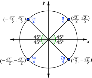
Using the fact that ![]() gives you the coordinates of the point in the first quadrant. Since the other points are reflections of this one, the coordinates have the same or the opposite values.
gives you the coordinates of the point in the first quadrant. Since the other points are reflections of this one, the coordinates have the same or the opposite values.
The diagram below can be used to find the values of ![]() and
and ![]() for
for ![]() . Note that because
. Note that because ![]() , when you draw the angle
, when you draw the angle![]() in standard position, you end up back at the x-axis.
in standard position, you end up back at the x-axis. ![]() radians or
radians or ![]() corresponds to the same point as 0 radians does, namely
corresponds to the same point as 0 radians does, namely ![]() .
.
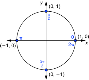
Using the coordinates of the four points gives you:

To become more familiar with the coordinates of points on the unit circle, try the following interactive exercise:
Our goal right now is to graph the function ![]() . Each point on this function’s graph will have the form
. Each point on this function’s graph will have the form ![]() with the values of
with the values of ![]() in radians. The first step is to gather together in a table all the values of
in radians. The first step is to gather together in a table all the values of ![]() that you know. To start we will use values of θ between 0° and 180°
that you know. To start we will use values of θ between 0° and 180° ![]() .
.
|
|
|
|
|
| 0° | 0 | 0 |
|
| 30° |
|
|
|
| 45° |
|
|
|
| 60° |
|
|
|
| 90° |
| 1 |
|
| 120° |
|
|
|
| 135° |
|
|
|
| 150° |
|
|
|
| 180° |
| 0 |
|


When we graph functions, we often say to graph the function on an interval. We use interval notation to describe the interval. Interval notation has the form ![]() , which means the interval begins at a and ends at b. In the example, the notation
, which means the interval begins at a and ends at b. In the example, the notation ![]() has the same meaning as
has the same meaning as ![]() .
.
| Example | ||
| Problem | Graph the sine function on the interval | |
|
|
| Plot all the points from the last column of the table above. Note that |
| Answer | The values increase from 0 to 1 and then decrease from 1 to 0. | |
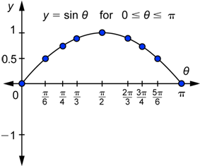
Note that our input is ![]() , the measure of the angle in radians, and that the horizontal axis is labeled
, the measure of the angle in radians, and that the horizontal axis is labeled ![]() , not x. Next we will gather together all the values of
, not x. Next we will gather together all the values of ![]() that you know for
that you know for ![]() in one table.
in one table.
|
|
|
|
|
| 180° |
| 0 |
|
| 210° |
|
|
|
| 225° |
|
|
|
| 240° |
|
|
|
| 270° |
|
|
|
| 300° |
|
|
|
| 315° |
|
|
|
| 330° |
|
|
|
| 360° |
| 0 |
|


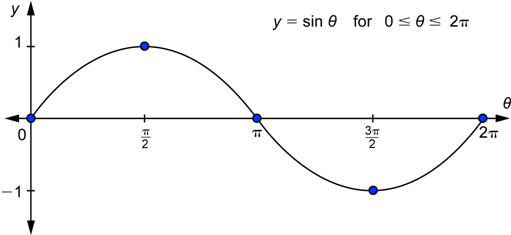
You could simply plot all the points from the last column and continue the graph in the last example. But notice the following: the values in the third column (or y-coordinates of the points) have the opposite values of the points that we just graphed. This means that instead of plotting points above the ![]() -axis, you will be plotting points below the
-axis, you will be plotting points below the ![]() -axis. Also, the inputs and outputs are spaced out in the same fashion for this part of the graph as they were for the first part of the graph. So instead of having a “hill” that goes from 0 up to 1 and down to 0, you will have a “valley” that goes down from 0 to
-axis. Also, the inputs and outputs are spaced out in the same fashion for this part of the graph as they were for the first part of the graph. So instead of having a “hill” that goes from 0 up to 1 and down to 0, you will have a “valley” that goes down from 0 to ![]() and then up to 0.
and then up to 0.
We have used values of θ from 0 to 2π to draw the graph of the sine function. What does the graph look like if we continue to the right of 2π for ![]() , which is one more time around the unit circle? In terms of degrees, these are angles between 360° and 720°. Let’s go back and look at one of these angles in standard position with the unit circle. A 400° angle is shown below.
, which is one more time around the unit circle? In terms of degrees, these are angles between 360° and 720°. Let’s go back and look at one of these angles in standard position with the unit circle. A 400° angle is shown below.
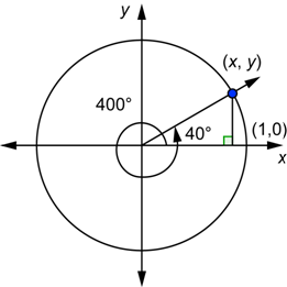
Because ![]() , the angle travels a full rotation plus another 40°, as shown by the curved arrow in the diagram. Imagine you are on (1, 0) and you walk around the circle one complete time and then you walk a little more to end up at (x, y). This point where the terminal side intersects the unit circle is the same point that you would get for a 40° angle. All of the trigonometric functions for these two angles are computed using the coordinates of this point. This means that
, the angle travels a full rotation plus another 40°, as shown by the curved arrow in the diagram. Imagine you are on (1, 0) and you walk around the circle one complete time and then you walk a little more to end up at (x, y). This point where the terminal side intersects the unit circle is the same point that you would get for a 40° angle. All of the trigonometric functions for these two angles are computed using the coordinates of this point. This means that ![]() ,
, ![]() ,
, ![]() , and the same is true for the three reciprocal functions.
, and the same is true for the three reciprocal functions.
There is nothing special about 400°. You could draw other angles that are greater than 360° and find similar results. The results above for sine and cosine can be rewritten as ![]() and
and ![]() . In general, it is true that
. In general, it is true that ![]() and
and ![]() , or, using radians:
, or, using radians:
![]()
These two equations tell us that when we go around the circle a second time, we are going to get the same values for ![]() as we did for
as we did for ![]() and the same values for
and the same values for ![]() as we did for
as we did for ![]() . In other words, as we go around the same circle a second time, at the same locations on the circle we will get the same values for the y-coordinate and the x-coordinate that we did the first time around the circle.
. In other words, as we go around the same circle a second time, at the same locations on the circle we will get the same values for the y-coordinate and the x-coordinate that we did the first time around the circle.
| Example | |
| Problem | Sketch the graph of the sine function on the interval |
|
| Because the values of the sine function between
The range is the set of all y-values that the function can have, so the range of
|
| Answer |
The range of |
The same reasoning that we used above works for negative angles. For example, the angles ![]() and 135° are drawn in standard position with the unit circle below.
and 135° are drawn in standard position with the unit circle below.
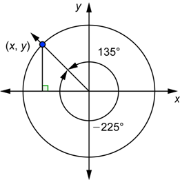
Because they are coterminal angles, they intersect the unit circle at the same point and therefore have the same coordinates. Therefore, ![]() ,
, ![]() , and so on for the other trigonometric functions. Notice that we could rewrite the first equation as
, and so on for the other trigonometric functions. Notice that we could rewrite the first equation as ![]() . Likewise,
. Likewise, ![]() , or
, or ![]() , is true for any angle
, is true for any angle ![]() including negative angles. The equation
including negative angles. The equation ![]() tells us that each time we go one additional full revolution around the circle we get the same values for the sine and the cosine as we did the first time around the circle.
tells us that each time we go one additional full revolution around the circle we get the same values for the sine and the cosine as we did the first time around the circle.
| Example | |
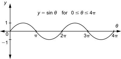
| Problem | Sketch the graph of the sine function on the interval |
|
|
Because
Therefore, the shape of the graph between |
| Answer |
|
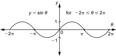
Since the equation![]() is true for any angle, it is an identity. We can use this identity to continue the graph of the sine function in either direction. This “hill and valley” pattern over an interval of length
is true for any angle, it is an identity. We can use this identity to continue the graph of the sine function in either direction. This “hill and valley” pattern over an interval of length ![]() will continue in both directions forever.
will continue in both directions forever.
Each time we add 2π to an angle, say ![]() , we will get the same function value.
, we will get the same function value.
![]()
You can also use the identity above to simplify calculations of the sine function by repeatedly subtracting ![]() from the angle. For example:
from the angle. For example:
![]()
| What is the value of
A) B) C) D)
|
Now our goal is to graph ![]() . We will go through the same procedure as we did for the sine function, and the result will be similar.
. We will go through the same procedure as we did for the sine function, and the result will be similar.
Each point on the function’s graph will have the form ![]() with the values of
with the values of ![]() in radians. The first step is to gather together in a table all the values of
in radians. The first step is to gather together in a table all the values of ![]() that you know. To start we will use values of θ between 0° and 180°
that you know. To start we will use values of θ between 0° and 180° ![]() .
.
|
|
|
|
|
| 0° | 0 | 1 |
|
| 30° |
|
|
|
| 45° |
|
|
|
| 60° |
|
|
|
| 90° |
| 0 |
|
| 120° |
|
|
|
| 135° |
|
|
|
| 150° |
|
|
|
| 180° |
|
|
|


| Example | ||
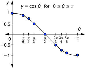
| Problem | Graph the cosine function on the interval | |
|
|
| Plot all the points from the last column of the table above. Note that |
| Answer | The values decrease from 1 to 0 and also continue to decrease from 0 to | |
Once again, our input is ![]() , the measure of the angle in radians, and the horizontal axis is labeled
, the measure of the angle in radians, and the horizontal axis is labeled ![]() , not x. Next we will gather together all the values of
, not x. Next we will gather together all the values of ![]() that you know for
that you know for ![]() in one table.
in one table.
|
|
|
|
|
| 180° |
|
|
|
| 210° |
|
|
|
| 225° |
|
|
|
| 240° |
|
|
|
| 270° |
| 0 |
|
| 300° |
|
|
|
| 315° |
|
|
|
| 330° |
|
|
|
| 360° |
| 1 |
|


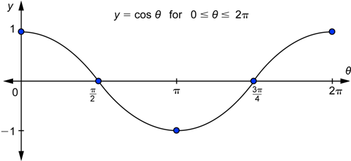
Again, you could simply plot all the points from the last column and continue the graph. Instead, compare the values in the third columns of the two tables: they are the same numbers, but in the reverse order. These are the y-coordinates of the points. This means that while the first part that we graphed decreased from 1 down to ![]() , this second part that we are graphing will increase from
, this second part that we are graphing will increase from ![]() to 1 and have the “same shape” (turned around the other way). Here it is:
to 1 and have the “same shape” (turned around the other way). Here it is:
The next step is to continue the graph for input values ![]() . When we were in the process of graphing the sine function, we established the following identity:
. When we were in the process of graphing the sine function, we established the following identity:
![]()
This equation tells us that when we go around the circle a second time, we are going to get the same values for ![]() as we did for
as we did for ![]() .
.
In other words, as we go around the same circle a second time, at the same locations on the circle we will get the same values for the x-coordinate that we did the first time around the circle.
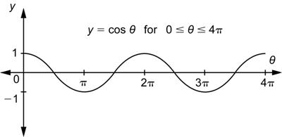
| Example | |
| Problem | Sketch the graph of the cosine function on the interval |
|
| Because the outputs between |
| Answer |
|
Just as the identity ![]() is true for negative angles, the identity
is true for negative angles, the identity ![]() is also true for any negative angle
is also true for any negative angle ![]() .
.
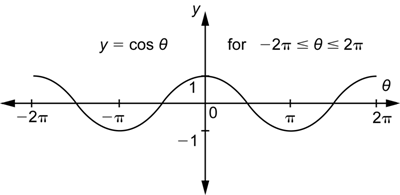
| Example | |
| Problem | Sketch the graph of the cosine function on the interval |
|
|
Because
Therefore, the shape of the graph between |
| Answer |
|
The identity ![]() was used above to extend the graph of the cosine function to the right and to the left. You can use this to continue to extend the graph in both directions. You will get another “hill and valley” pattern that repeats after intervals of length
was used above to extend the graph of the cosine function to the right and to the left. You can use this to continue to extend the graph in both directions. You will get another “hill and valley” pattern that repeats after intervals of length ![]() in both directions.
in both directions.
Another important feature of the graph of ![]() is that the left and right halves are mirror images of each other over the y-axis. The graph of
is that the left and right halves are mirror images of each other over the y-axis. The graph of ![]() has this same property. Another way to describe this is to say that if you substitute a number and its opposite into the function, you will get the same value as the previous equation. For example,
has this same property. Another way to describe this is to say that if you substitute a number and its opposite into the function, you will get the same value as the previous equation. For example, ![]() ,
, ![]() , or in general,
, or in general, ![]() . We say that the graph is symmetric about the y-axis. The diagram below shows two points taken from a symmetric graph.
. We say that the graph is symmetric about the y-axis. The diagram below shows two points taken from a symmetric graph.
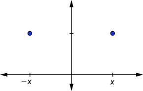
The height of the points at opposite inputs is the same. The height is the value of the function. A function whose graph is symmetric about the y-axis has ![]() .
.
| What is the range of the cosine function?
A) all values in the interval B) all values in the interval C) all values in the interval D) all real numbers
|
The graphs of sine and cosine both have hills and valleys in a repeating pattern.
Since this repeating pattern can be extended indefinitely to the left and right, the domain for both functions is the real numbers. The range for both of them is the interval ![]() .
.
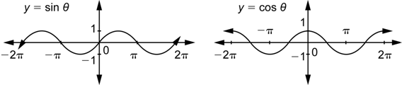
Let’s now compare these graphs in some other ways.
First we want to see what happens to the graph of a function when you change the input by adding a constant to it. Compare ![]() and
and ![]() . Here is a table with some values for these two functions.
. Here is a table with some values for these two functions.
|
|
|
|
|
| 0 | 0 |
| 1 |
|
|
|
|
|
|
|
|
|
|
|
|
|
|
|
|
| 1 |
| 0 |
|
|
|
|
|
|
|
|
|
|
|
|
|
|
|
|
| 0 |
|
|
Now we’ll graph these two functions. As a reminder, the input is ![]() for both of these functions. To graph
for both of these functions. To graph ![]() , you use the numbers in the first and second columns. To graph
, you use the numbers in the first and second columns. To graph ![]() , you use the numbers in the first and fourth columns. (The third column was just written as a convenient intermediate step. You do not use that for the graph.)
, you use the numbers in the first and fourth columns. (The third column was just written as a convenient intermediate step. You do not use that for the graph.)
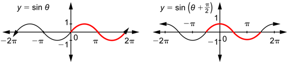
First observe, as shown by the pieces in red, that the effect of adding ![]() to the input is to shift the graph to the left by
to the input is to shift the graph to the left by ![]() units. You may recall seeing this effect when you graphed radical functions such as
units. You may recall seeing this effect when you graphed radical functions such as ![]() and
and ![]() (adding the 1 to the input shifted the graph of
(adding the 1 to the input shifted the graph of ![]() to the left 1 unit). In general, if you add a positive constant c to the input of a function, that will have the effect of shifting the original graph to the left by c units. If you subtract a positive constant c from the input of a function, that will have the effect of shifting the original graph to the right by c units.
to the left 1 unit). In general, if you add a positive constant c to the input of a function, that will have the effect of shifting the original graph to the left by c units. If you subtract a positive constant c from the input of a function, that will have the effect of shifting the original graph to the right by c units.
Next observe that the graph on the right is already familiar to you. It is the graph of ![]() ! So you can say that the graph of
! So you can say that the graph of ![]() is the same as the graph of
is the same as the graph of ![]() , or you can say that the graph of
, or you can say that the graph of ![]() shifted to the left by
shifted to the left by ![]() units is the graph of
units is the graph of ![]() .
.
The next example looks at a shift in the other direction.
| Example | |
| Problem | Sketch the graph of How does the graph compare to the graph of |
|
| The graph of |
|
|
|
| Answer | The graph of |
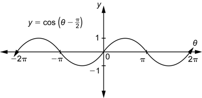
Because the patterns repeat, you could start with the graph of either sine or cosine and shift it by different amounts to the right or left to get the graph of the other function.
| Which comparison of the graphs of
A) They are the same. B) The graph of C) The graph of D) The graph of
|
For practice graphing sine and cosine, try the following interactive exercise:
Summary
The graphs of sine and cosine have the same shape: a repeating “hill and valley” pattern over an interval on the horizontal axis that has a length of ![]() . The sine and cosine functions have the same domain—the real numbers—and the same range—the interval of values
. The sine and cosine functions have the same domain—the real numbers—and the same range—the interval of values ![]() .
.
The graphs of the two functions, though similar, are not identical. One way to describe their relationship is to say that the graph of ![]() is identical to the graph of
is identical to the graph of ![]() shifted
shifted ![]() units to the left. Another way to describe their relationship is to say that the graph of
units to the left. Another way to describe their relationship is to say that the graph of ![]() is identical to the graph of
is identical to the graph of ![]() shifted
shifted ![]() units to the right.
units to the right.
